This is a guest article by Andrea Delgado, Daniel Calegari, and Nicolás Carignani from the Computer Science Institute, School of Engineering, Universidad de la República, Uruguay. They have used open data to discover the process flows from bus lines in Montevideo. They then exported the XML process maps from Disco to display the discovered processes in the spatial city map. In this article, they explain their approach and give you all their scripts and the information that you need to reproduce the approach for your own city.

If you have a guest article or process mining case study that you would like to share, please get in touch with us via anne@fluxicon.com.

Urban mobility allows us to access housing, jobs, and urban services, and its planning, control, and analysis are of utmost importance to city governments. Transport modeling and planning must address several challenges, such as traffic congestion, public transport crowding, pedestrian difficulties, and atmospheric pollution. Smart cities use technology to improve urban services, e.g., Intelligent Transportation Systems that incorporate technologies generating real-time data that can be processed to extract valuable information.

In 2010, the Municipality of Montevideo, Uruguay, defined a Mobility Plan, which included the creation of the Metropolitan Transportation System (Sistema de Transporte Metropolitano, STM), serving a population of 1.4 million. The STM defines several city public transportation elements, adding an ITS with on-board GPS unit control systems on each bus and smart cards for citizens, as illustrated in Figure 1. The Mobility Management Center manages and controls traffic and transportation in the city using the real-time data provided by the STM.

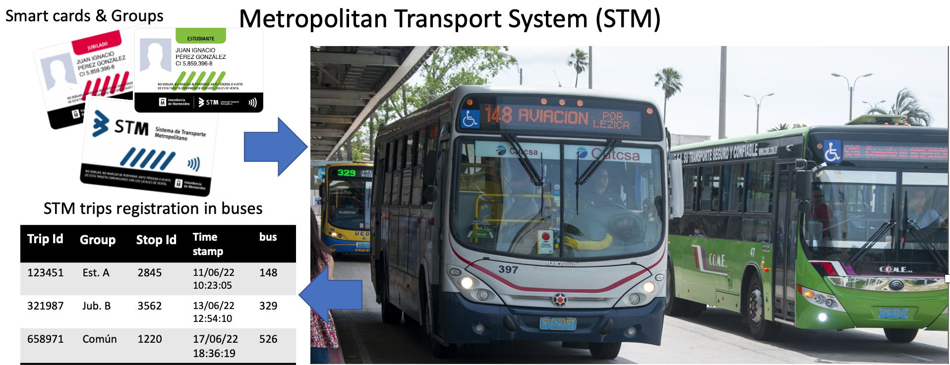
Fig. 1: STM system elements: smart cards for citizens, buses with GPS, and smart card readers that register data for each trip.

We address a set of questions defined by the Municipality of Montevideo in the context of a joint research project concerning their transportation system (STM) data from buses and smart card trips by applying process mining techniques. For this, we use open data provided by the STM within the governmental open data catalog¹. We provided another view on public transportation data to business experts to help them make decisions on the city’s urban mobility, considering different perspectives, including the behavior of bus lines according to the planned routes [1].

People working in the urban mobility domain are used to analyze data in traditional formats (tables, graphics, etc.) and locate geospatial data in the city map. In our first attempt, we analyzed the reference process model corresponding to the bus routes and the data from the actual trips made by passengers within the buses using a traditional process mining approach. However, we realized that the results could be deployed over Montevideo´s city map to improve visualization and understanding of the outcomes.

In what follows, we present an extract of the behavior of bus lines analysis presented in [1], focusing on deploying the bus lines process models provided by Disco over Montevideo´s city map using the open-source geospatial software QGis².

Open Data from the STM system

Below, we present some definitions of the Metropolitan Transport System (STM) that are needed to understand the data we used for the analysis:

• A line is a public name by which a set of routes of a transportation company is known, e.g., 2, 103, 148, 306, 405, 526, D11.
• Sub-lines are each one of the routes that a line has (difference in the streets traveled), with a direction.
• A variant is each instance of the route of a sub-line, with a specific origin, destination, and direction (maximal, partial, circular)
• Every variant (line, sub-line, direction, origin, destination) has a set of frequencies that defines a departure time on a given day (working days, Saturdays, Sundays, and holidays).
• Stops in the route of each variant are known, as well as the stop of origin and destination, all identified by a unique code.

The theoretical schedule by which a bus travels through each stop is also known for each frequency. Apart from the bus data, the information on passengers’ STM card payments is also known. There are different types of passengers, e.g., ordinary users, retirees, and students. Every time a payment is recorded, there is a registry with the kind of passenger, the stop at which it boards, the variant and frequency to which the bus belongs, and the time of departure, among other information. Below, we present the primary datasets we used for the reference process models of the bus line routes and the process model of actual passengers’ trips we show in the map of Montevideo, extracted from [1].

[UBS] Urban bus schedules, by stop³. It contains the bus schedules for urban transportation. These are estimated theoretical schedules in which a bus line will pass through a particular stop along its route. These data are obtained by estimating each stop’s passing times according to the transport units’ average speed, predefined schedule, and distance between stops.

• type of day: 1 - working days (Monday to Friday), 2- Saturdays, 3 - Sundays and holidays.
• cod variant: identifies the variant of the line.
• frequency: identifies the frequency for the variant for the type of day, i.e., the specific hours.
• cod loc stop: shows the code of each stop
• ordinal: shows the number of stops within the bus line route, i.e., first (1), second (2), etc.
• hour: shows the estimated hour for the bus to arrive at the stop
• day before: indicates if the frequency started the day before (for late-night lines)

The UBS file contains data from more than 100 bus lines with more than 800 variants and 1000 corresponding frequencies. Four companies provide the service and cover the metropolitan area with more than 4700 stops.

[TSB] Trips made on STM buses⁴. It contains all the trips made on the urban collective transport lines in Montevideo by each operating company, line, variant, day and time, tickets sold at all stops in the system, by type of user, payment method, and sections of each trip. The information comes from all the records processed by the STM trip validation machines.

• id trip: identifies the trip within the system; in combined tickets, the id trip is repeated in all
• buses the user rides while the ticket is valid.
• line code: shows the code of the bus line
• cod variant: identifies the variant of the line
• frequency: identifies the frequency for the variant
• with card: shows if the STM card was used in the payment of the trip
• date event: timestamp of date and hour of the trip
• trip type: combined (1 hour, 2 hours), student, retired, standard user.
• origin stop code: shows the code of the stop at which the user got on the bus

The TSB file we used to analyze the STM trips corresponds to May 2022, which contains 25 million records, including all trips from the STM system registered within the 136 bus lines of Montevideo. For experimentation, we selected different bus lines from these to maximize the city coverage [1].

[BLOD]⁵ Bus lines, origin, and destination. It contains geographic information that, among other data, includes the lines’ description, origin, and destination. This dataset contains the shapefile⁶ that provides geospatial data for the bus line destinations for each bus line, sub-line, and variant.

[CTSC]⁷ Buses: stops and checkpoints. It contains geographic information on stops and control points. This dataset contains the shapefile with geospatial data for the stops defined within the city, referenced in the bus lines routes.

Process mining applied to urban mobility

From the perspective of the behavior of bus lines according to the planned routes, we analyzed the data to answer some of the business experts’ questions, in particular, the ones related to bus lines and their use by passengers:

1. What is the route of a bus line?
2. How is the mobility of people within the STM?

Regarding the reference model of the bus lines (question 1), we can obtain it from the UBS file that contains the theoretical schedules. We select variants for each line, setting the variant and frequency codes and day as {case ID}, the stop code as {activity ID}, the hour of the stop as {timestamp}, and the rest of the data fields as {attributes} of the activity. Since variants have different directions corresponding to the sub-line, we obtain two sequential sections in each direction. The reference model must contain the same stops in the same order as the ones defined by the variant in the STM system, which is accessible from the website for a scheduled consultation.

Regarding users’ data on authentic trips of the bus lines (question 2), we can discover a travel model for a bus line from the TSB file. We filter by line and selected the variant, frequency, and day of the trip as {case ID}, the stop code as {activity ID}, the hour of each trip of each stop as {timestamp}, and the rest of the data fields as {attributes} of the activity. The number of events at each stop is the number of passengers boarding. Thus, loops represent multiple passenger boardings at the same stop. Unlike the reference model, the process is not linear since, in some frequencies, there are stops in which nobody boards. We can filter data by days (business days, Saturdays, Sundays, and holidays), day hours, seasons, type of user, company, etc.

Figure 2 (extracted from [1]) depicts examples of these two process models discovered in Disco for bus line 125, variant 667, which is the maximal variant in one direction. This bus line goes in one direction from the old city to the West, ending in Cerro Beach and returning in the other direction.

In this Figure, we can see: a) the bus line in the map taken from the STM schedules site⁸, b) an excerpt of the reference model (i.e., bus stops included in the line), and c) an excerpt of the STM trips within its frequencies.

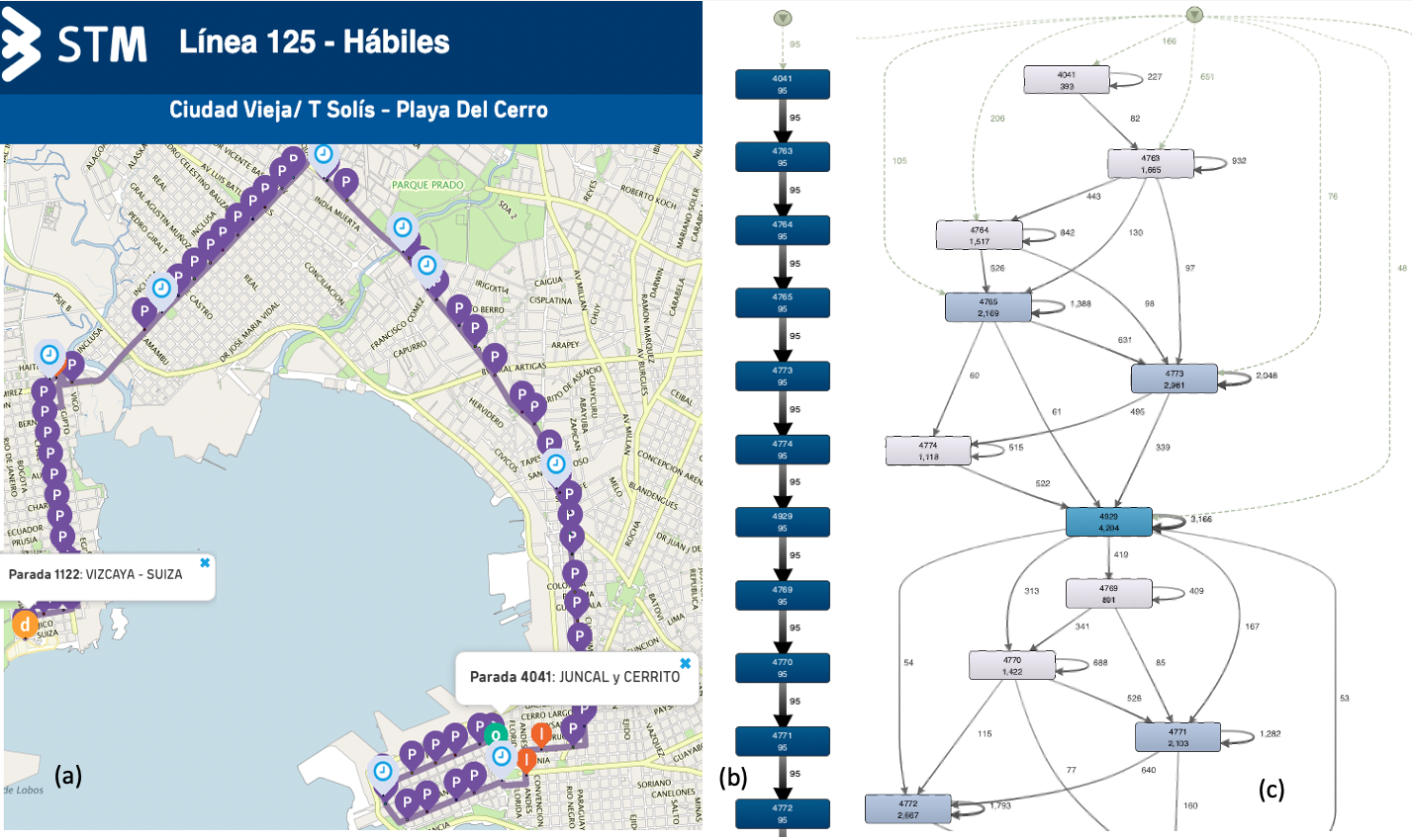
Fig. 2: Bus line 125 route from [1] with stops for the 667 variant: a) in the STM website bus schedule, b) excerpt of the reference model, and c) excerpt of the STM trips within its frequencies

From users’ data on actual trips of the bus lines (question 2), it could be possible to analyze load metrics after filtering and discovering the model. For example, it is possible to answer: At which stops do people not get on? At which stops do more people get on? At what times does the bus have more and fewer passengers? What happens to those lines in a particular area? Moreover, it is possible to answer performance questions such as: What is the total duration of the frequencies (on average, maximum, minimum)? Are there frequencies with delays? As an example, we present in Figure 3 the performance model for bus line 300 (one of its variants), which goes from the bottom of the city near the city center to the city’s north periphery, showing the delays in the transitions between stops of the bus line route, calculated with the actual trips data.

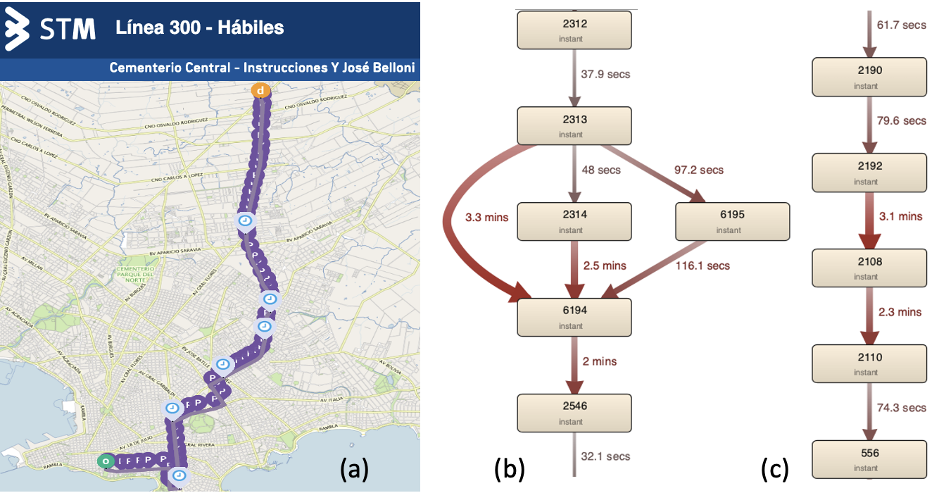
Fig. 3: Bus line 300 route with stops for one of its variants: a) in the STM website bus schedule, b) and c) excerpt of performance models with delays in the transitions from the STM trips data.

Exporting from Disco and visualizing the models over Montevideo´s city map

As mentioned before, people working in the urban mobility domain are used to seeing locations on the city map, analyzing data, and considering geospatial data. Although the process models provided valuable information, they should be compared manually to the bus line route provided over the STM site’s city map to identify where some behaviors arise. To improve visualization for business experts, we developed a prototype to deploy process models over Montevideo’s city map.

Disco allows the export of XML files of the resulting process models, both the process map and the performance view. As we selected the bus line stops as activities of the process, which have a corresponding geospatial location over Montevideo city, we can locate each stop in the map and, correspondingly, the Disco process model we exported. Also, the dataset containing the data for each bus line route destination is used to locate the reference bus line route over the map. These data correspond to BLOD and CTSC files with shapefiles geospatial data of the bus line routes and stops in Montevideo.

We used the open-source geospatial software QGIS, which supports loading city maps with corresponding coordinates worldwide, creating/adding layers with geospatial data in the shapefiles to be seen over the map, and developing scripts with Python to work with them. In Figure 4, we present the process flow for deploying the process models exported from Disco over the city map loaded in QGis with the help of the scripts we developed.

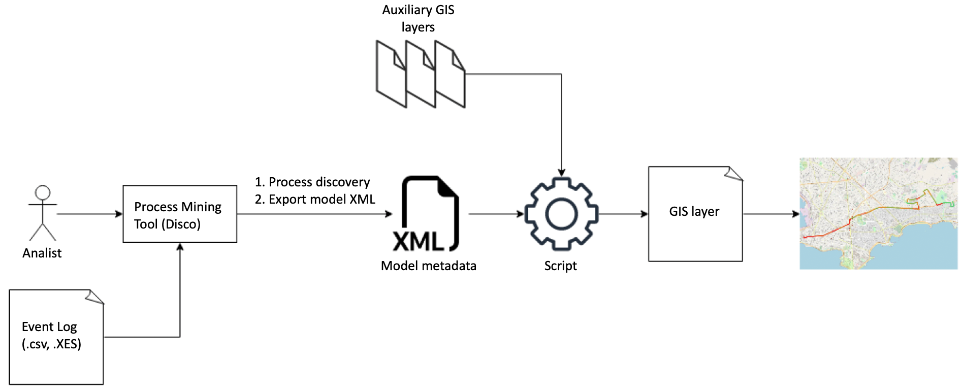
Fig. 4: Process for deploying process models exported from Disco over the city map in QGis.

The first step is to load the event log into Disco, in our case, the data corresponding to the passengers’ actual trips over a bus line, to discover the corresponding process model of the bus line route, which can be filtered by variant as shown above. Then, the resulting process model can be exported in XML format, which will be one of the inputs to QGis to show over the city map. We want to show both the process map with the flow of the actual trips over the bus line and the performance map with the delays of the buses on the actual trips, as depicted in Figures 2 and 3. In Fig. 5 a screenshot of the export model XML we used in Disco is shown.

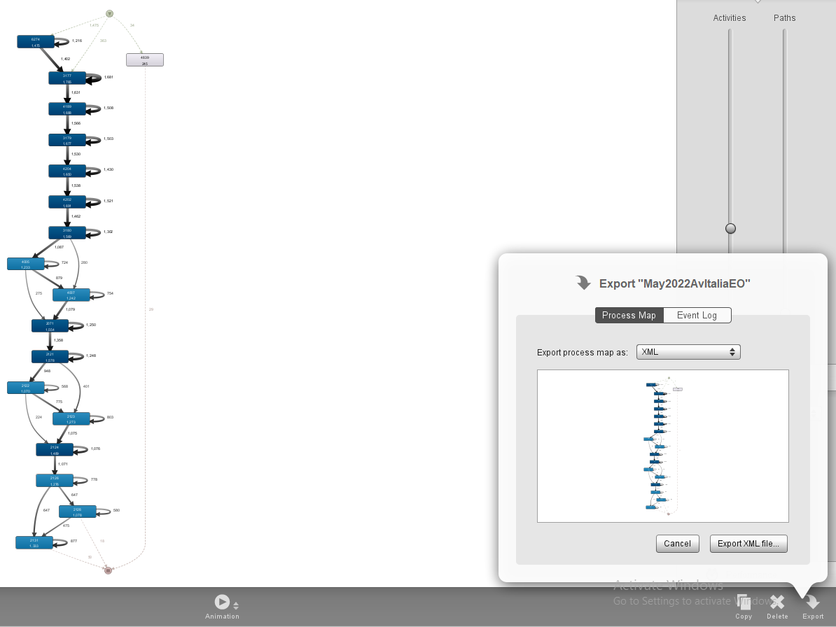
Fig. 5: Disco export model in XML format

In QGis, we first load the shapefile data of the stops and the origin and destination of buses over the city map as vector layers and then the city map layer as the XYZ layer. These layers should be in the same coordinate format and time zone to match locations. We load the Python scripts we developed in the project options. Figure 6 shows a QGis screenshot with the three layers in the bottom left panel and the Python scripts in the right panel.

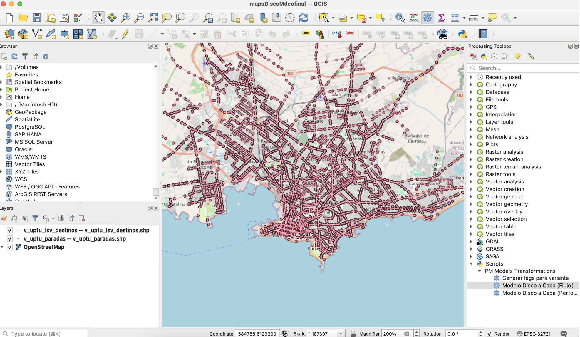
Fig. 6: QGis software with Montevideo city map layer (XYZ), bus stops over the city (from CTSC shapefile), and bus lines origin and destination over stops (from BLOD shapefile)

The Python scripts we developed transform the Disco process models into a QGis layer that can be deployed over the city map, using as reference the stops and the bus line origin and destination geospatial data we first loaded over the city map. The QGis scripts are as follows:

• layer_from_disco_model_flow.py: transforms a Disco process model flow (XML) into a QGIS layer, which allows visualization over the map.
• legs_for_variant.py: divides a bus line into sections (consecutive stops), which is then used as input for the performance process model calculations.
• layer_from_disco_model_performance.py: transforms a Disco performance process model (XML) into a QGIS layer using the legs_for_variant output layer as input.

To illustrate the process in QGis and its results, we use the bus line 21 route that we show in Figure 7 for the 7488 variant: a) the bus line in the map taken from the STM schedules site, and b) an excerpt of the STM trips within its frequencies, which is the one we import in QGis. This bus line goes in one direction from Independence Square (the entrance of the old city) to the east, parallel to the coast, and ends in the Portones Shopping Center in the Punta Gorda neighborhood. It has extensions of the route to the old city (left) and to the entrance of the Canelones Department (right).

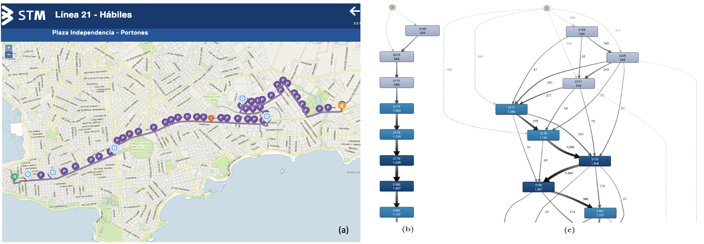
Fig. 7: Bus line 21 route with stops for the 7488 variant: a) in the STM website Bus schedule, b) excerpt of the reference model, and c) excerpt of the STM trips within its frequencies

The process model exported from Disco corresponding to Figure 7 c), and transformed into a QGis layer can be seen over the Montevideo city map shown in Figure 8, with zoom over the first sections (left). It can be seen that differently to the ones presented in Figure 7, a) and b), it has arcs that traverse over non-consecutive stops, which reflects, as we mentioned, the actual trips over the bus line route, where in some frequencies, no passengers are getting into the bus in some stops.

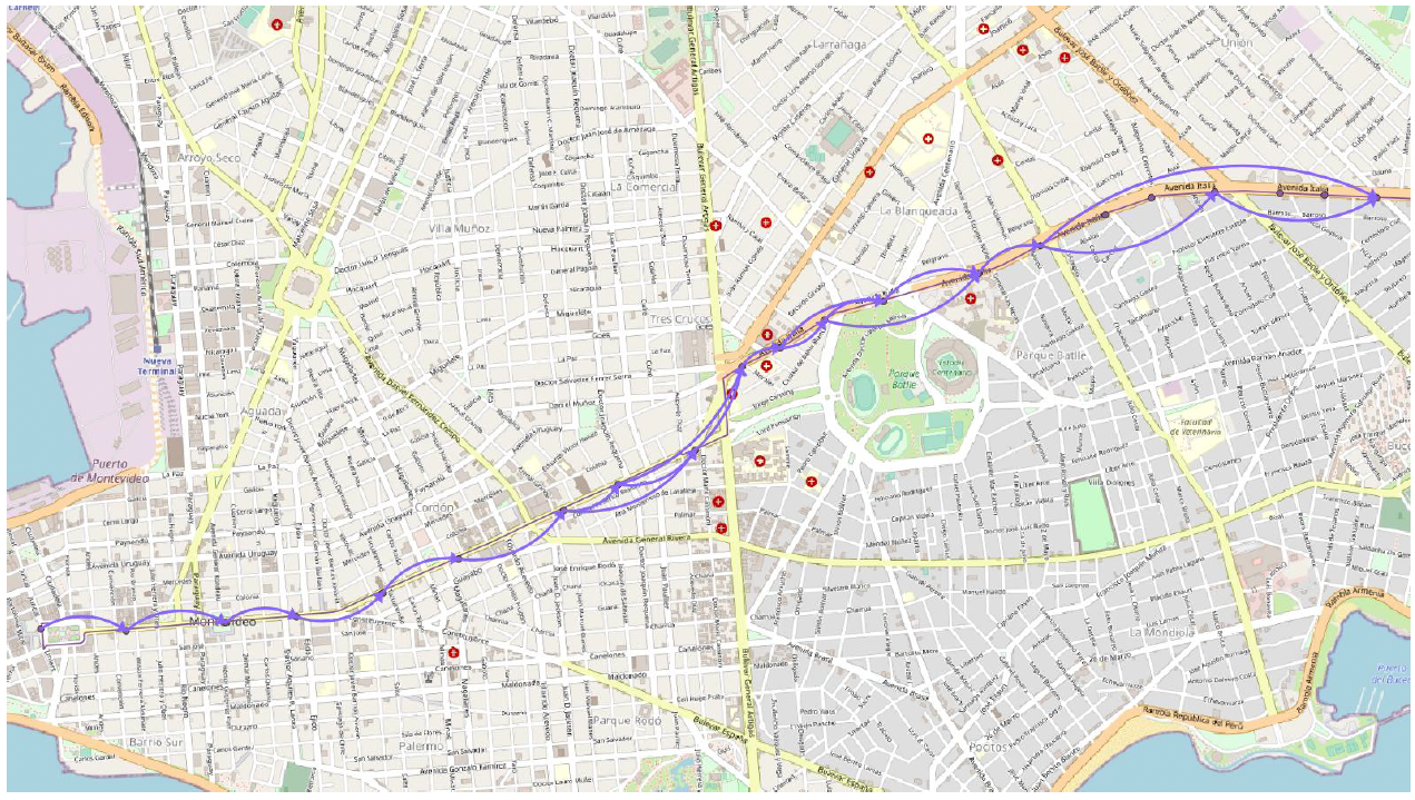
Fig. 8: Process model flow view exported from Disco discovered from the STM trips actual data for the 21 bus line route and variant 7488 deployed over Montevideo city map

Zooming again on the upper-right corner flow, we can see the details of the process model flow in Disco and the corresponding process model deployed over the city map, as shown in Figure 9: a) the process model in the city map, and b) the process model flow in Disco. It can be seen that stop 2126 goes over the left in the map, stop 2131 goes over the right, and stop 2128 goes in the middle, with the flow to the right. If the two views of the model are compared in Figure 9 a) and b), the difference is noticeable. The map gives a much greater context, allowing one to quickly know the exact location of the activities (stops in this case), the corresponding area, and the neighborhood, allowing one to relate the generated model to information not included.

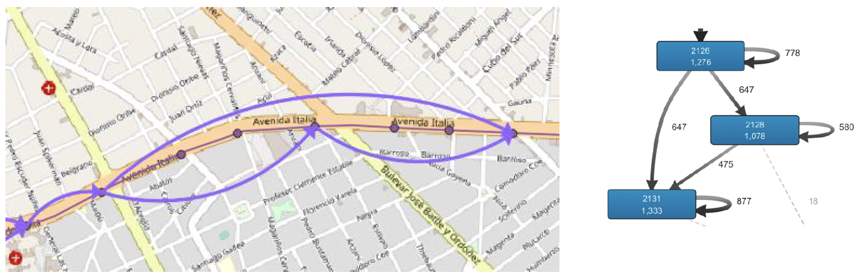
Fig. 9: Zoom of the process model of the bus line 21 route upper-right corner flow and correspondence with the Disco process map

In this case, we could further investigate why, on several occasions, no passengers are getting on the bus at stop 2128. Some causes could be the following: the stop infrastructure is worse than other nearby stops, there are security issues in the area, and it is mainly used by specific groups of users (e.g., students) within input and output hours of the school.

The performance process model exported from Disco corresponding to Figure 7 c), and transformed into a QGis layer can be seen over the Montevideo city map shown in Figure 10: a) the model exported from Disco with delays in transitions between the stops, and b) deployed in the map showing sections delays using the semaphore metaphor: green, yellow and red for more significant delays.

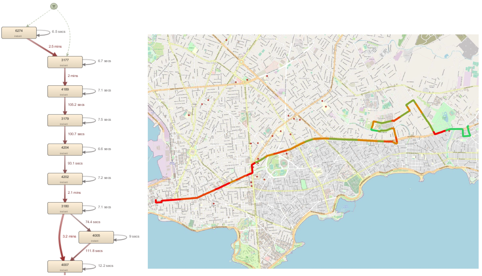
Fig. 10: Performance process model for the bus line 21 route from the bus actual trips data: a) the model exported from Disco with delays in transitions, and b) deployed in the map showing sections delays

Again, as in Figure 8, being able to visualize the specific sections of the bus line that present the worst times over the bus line route in the map, provides a much greater context, allowing to identify the zone at which the sections belong quickly. In this case, it can be seen that the section to the left that goes from the Centenario stadium (round green space marked in the middle below the bus line) to the old city presents the worst delays. This is consistent with that zone being bustling over Avenue Av. Italia, passing through the Three Crosses bus terminal and traversing from start to end the main center avenue Av. 18 de Julio towards the old city entrance (Independence Square).

Conclusions and reproducibility for other cities

We have presented a case study on the application of process mining to analyze urban mobility open data from the STM transport system in Montevideo, Uruguay. We showed how, using Disco, we can discover the reference process model of bus lines using the stops defined for each one and the actual STM trips process model that shows the actual behavior of bus lines regarding passengers’ use within the different frequencies (actual trips) of the buses.

Due to the interest of business people in this specific domain who normally visualize and analyze data over the city map, we developed a prototype that, using the process model export feature of Disco in XML format, allows us to import them into the open-source geospatial software QGis, deploying them over the city map of Montevideo. This provides much greater context to users, as discussed in the previous section.

Regarding reproducibility for other cities, exporting the process models to Disco, importing the layers for the stops and bus lines routes over the city map, and generating the QGis layers for the process models can be applied straightforwardly. For the scripts to work, the process models to be exported from Disco should use as activities the stops of the bus lines, and the files containing the shapefiles with geospatial data of the stops and bus lines routes should be available. The city map layer is loaded as an XYZ layer directly in QGis, available for all cities. The data and format are available from the bus actual trips system of the desired city (i.e., the records of the passengers’ trips) and should probably have to be manipulated to provide the same fields that we used (e.g., bus line, variant, stops to relate to the shapefiles, etc.), or the scripts can be adapted to the data provided by the system under analysis.

The scripts and data are publicly available⁹ for further experimentation and analysis.

References

[1] Delgado, A., Calegari, D., Process Mining for Improving Urban Mobility in Smart Cities: Challenges and Application with Open Data, 56th Hawaii International Conference on System Sciences (HICSS-56), Maui, Hawaii, USA, Scholarspace, 2023. https://hdl.handle.net/10125/102846

[2] Rodao, B., Carignani, N., Ferreira, S., Minería de Procesos para el análisis de movilidad urbana. Tesis de grado. Universidad de la República (Uruguay). Facultad de Ingeniería, 2023. (In Spanish) https://hdl.handle.net/20.500.12008/42549

Authors

Andrea Delgado - adelgado@fing.edu.uy - https://www.fing.edu.uy/~adelgado

Daniel Calegari - dcalegar@fing.edu.uy - https://www.fing.edu.uy/~dcalegar

Nicolás Carignani - nicolas.carignani@fing.edu.uy

Anne Rozinat

Market, customers, and everything else

• anne@fluxicon.com
• annerozinat
• @arozinat

Anne knows how to mine a process like no other. She has conducted a large number of process mining projects with companies such as Philips Healthcare, Océ, ASML, Philips Consumer Lifestyle, and many others.