When you perform a process mining analysis, then the discovered process map and the variants are only the starting point. You then want to dive deeper into the process based on the questions that you have about it.
One of the typical questions is about the performance of the process. For example, you may have a service level agreement (SLA) with respect to the overall throughput time of the process. Within Disco, you can analyze the case duration distribution and you can filter your data to focus on the slow cases to find out where in the process they lose so much time (see also the video at the top for a demonstration of how to do this).
Once you discover a bottleneck in your process, the animation is a very powerful tool to visualize the bottleneck to your co-workers. Rather than just giving them abstract statistics and charts, they can literally see where a lot of the cases are piling up and where the queuing occurs (see below). This will help you to explain your findings and engage them in discussions about how the process can be improved. As soon as a bottleneck has been resolved, you can focus on the next one to support a continuous improvement of your process.
Once you dig into the performance analysis for your process, there are two things to know that can be helpful. So, in this article, we want to give you these two tips that will help you perform better bottleneck analyses on your own data.
Tip No. 1: Consider the median instead of the mean
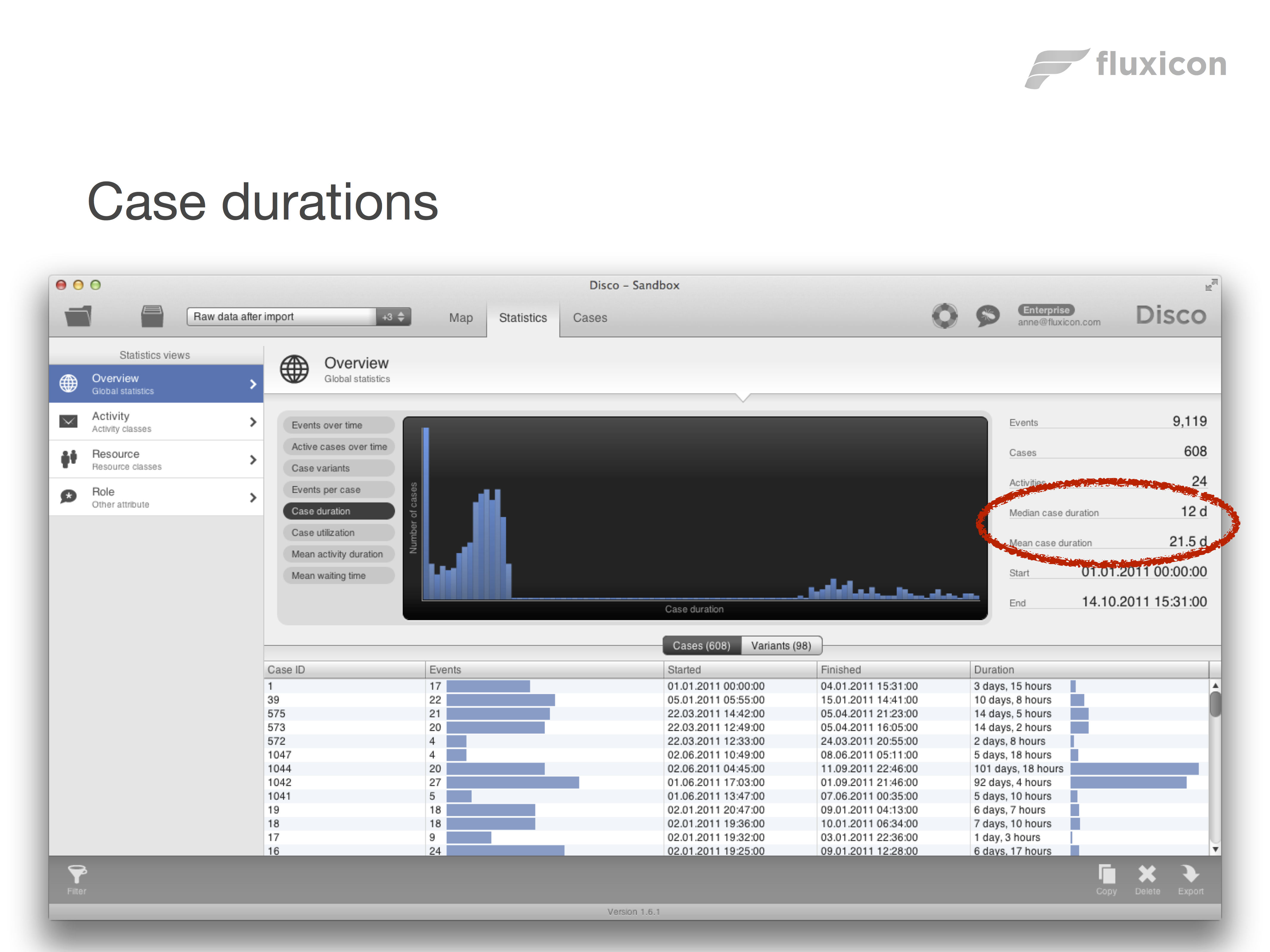
All the performance metrics in Disco, for example, the case durations, the activity durations, but also the performance metrics in the process map, give you both the mean and the median duration.
Often, there is quite a difference between the two. For example, if you look at the case duration below (click on the image to see a larger picture) then you will notice that the mean case duration is 21.5 days while the median case duration is just 12 days – That means the median case duration is almost half of the mean case duration for this process!
The reason that this can happen is that the mean is much more susceptible to outliers. To understand why, let’s take a look at how both the mean and the median are calculated. In the figure below, you can see seven measurements lined up according to their size. For example, these could be seven cases of which we have measured the throughput time: Two cases were measured with 1 day throughput time, one case was measured with 2 days throughput time, three cases were measured with 3 days throughput time, and one case – our outlier – had a throughput time of 30 days.
Now, the median is defined as the value in the middle of the lower 50% and the higher 50% of measurements. So, 3 would be the median value in this example, because half of the cases took longer (or equally long) and half of the cases were faster. In contrast, the mean or average value is calculated as the sum of all values divided by the number of values. So, the mean yields 6.14 in this example. The mean is more than twice as high compared to the median, because the mean is much more influenced by the one extreme case with the 30 days throughput time.

In practice, many processes have a distribution similar to the picture above. For example, your customer service process may typically take up to two weeks, but you have these few, very complicated cases that took one or two years to resolve. Or when a typical incident can be closed with 8-10 steps, there is this one extreme case that was ping-ponged between different groups more than 200 times.
In such processes, the median (also known as the 50th percentile) gives you a much better idea of the typical performance characteristics of a process than the arithmetic mean. Therefore, the median can often better point you to the places in the process that typically are quite slow. For example, from the mean durations visualized in the illustration below on the left, you can get the impression that basically the whole area on the left of the process is problematic in terms of performance. The median performance view, shown on the right, makes it clear that the bulk of the problems actually lies with one activity on the lower left.

Of course there are still situations, where you might want to use the mean. One reason can be that it is easier understood by people who are not statistically minded. Or your KPIs might be defined based on the mean, so you should use the mean for your analysis, too. But keep in mind that if you have a skewed distribution with heavy outliers, the mean can be misleading and the median will be a better metric to get a sense of what a typical value looks like.
Tip No. 2: Combine total duration with the median
The second tip that we want to give you is to keep in mind that neither the mean nor the median take the frequency into account. This can be a problem, because you want to focus your improvement efforts on those places in the process, where they can have the most impact.
For example, let’s take a look at the process map below. We have used the median for the performance visualization and it looks like that path that typically takes 5.6 days is the biggest problem.

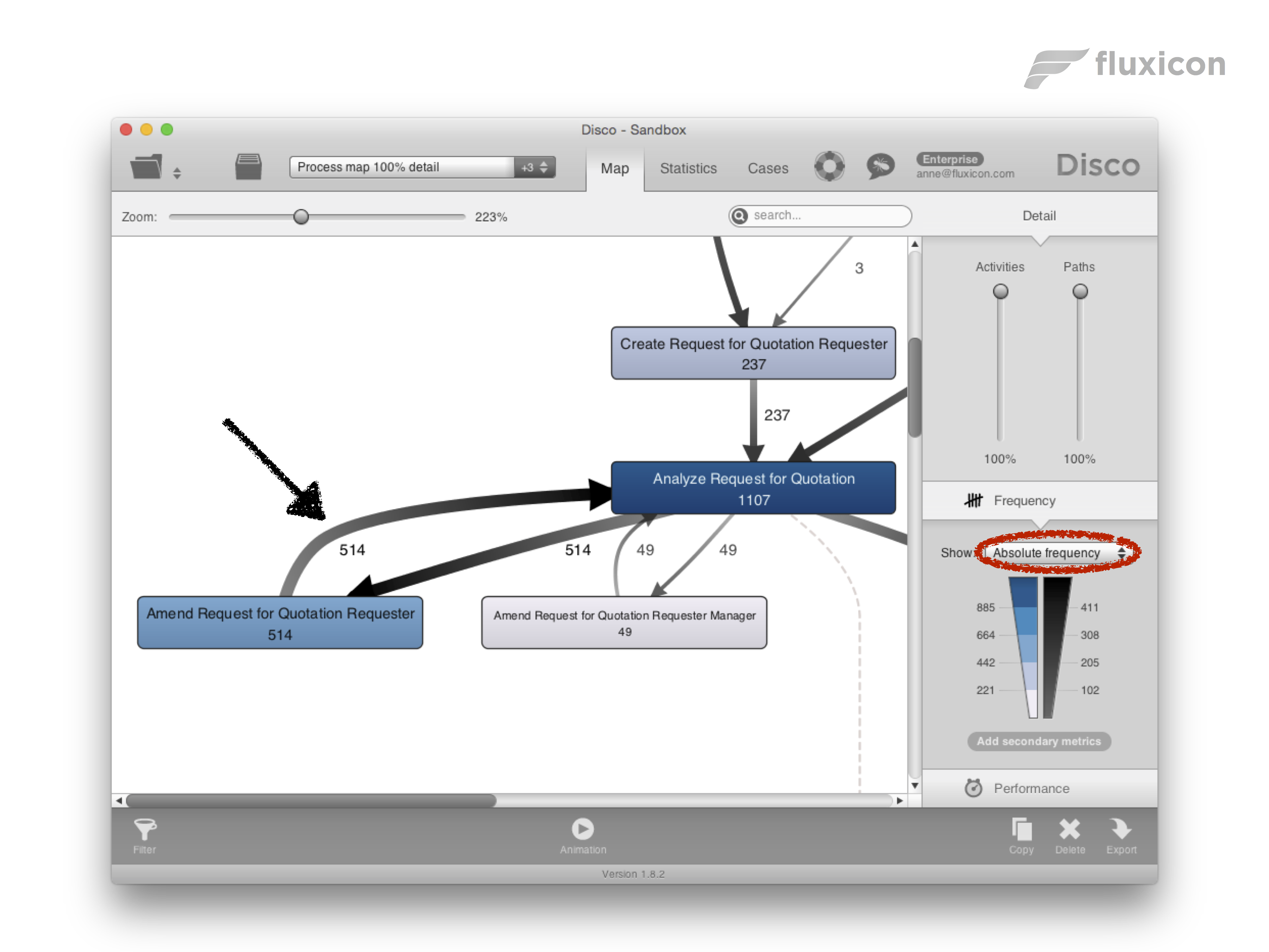
However, once we switch to the frequency view, we can see that the path right next to it is about 10 times as frequent. So, although the median delay on that path was just 3 days (instead of 5.6 days), the impact of improving this particular bottleneck will be greater.
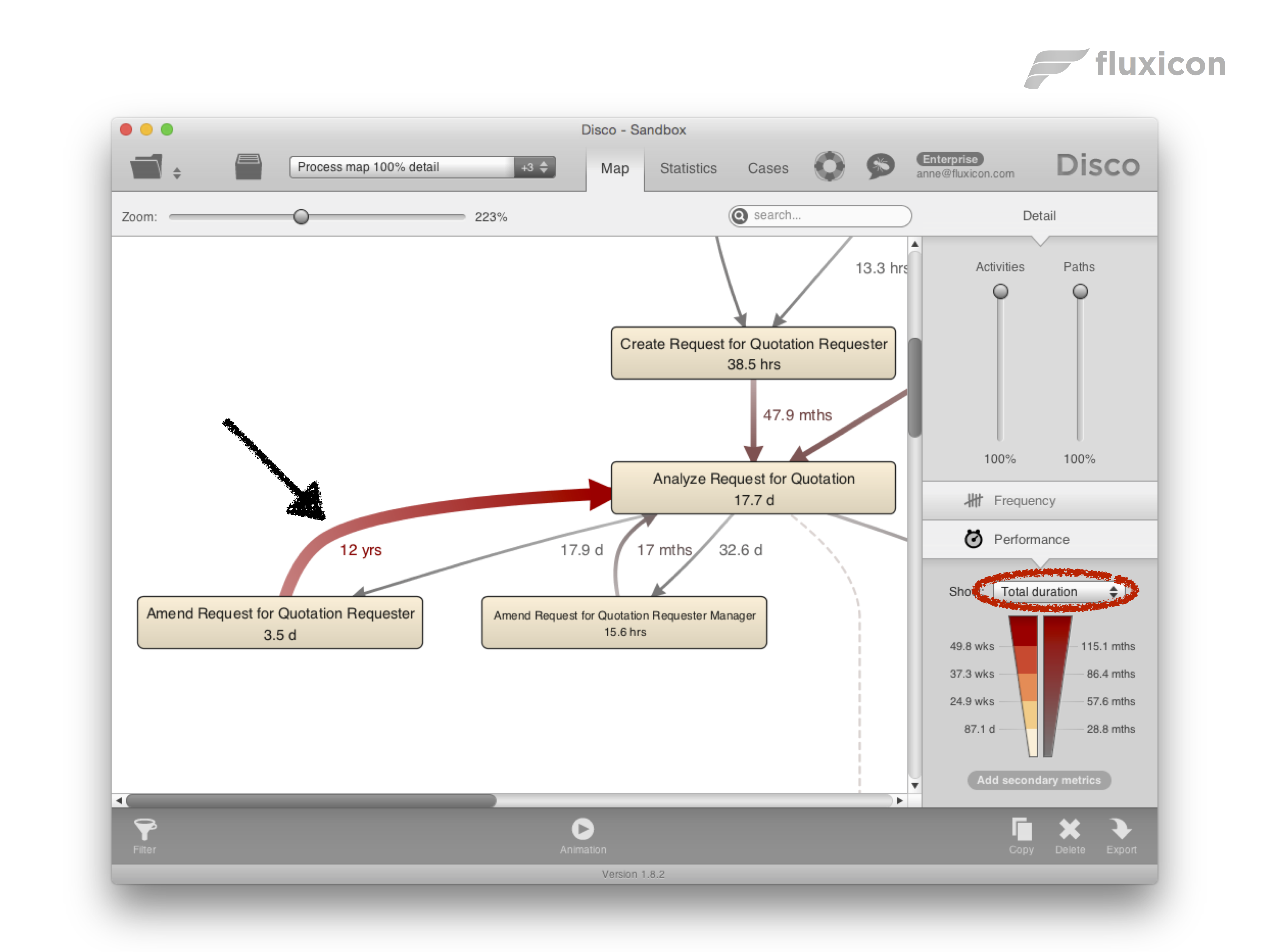
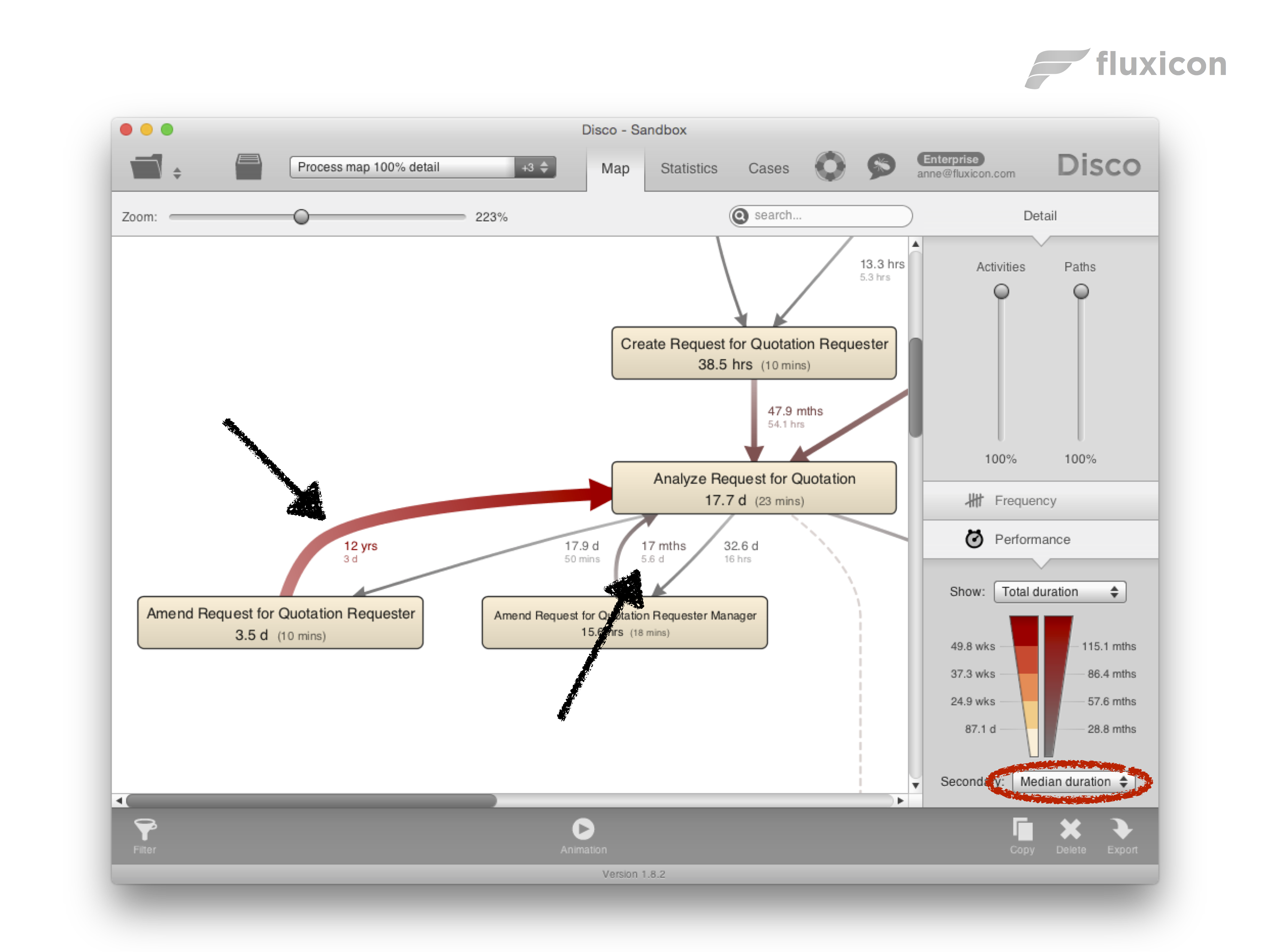
The best way to take the frequency into account in your bottleneck analysis is to use the total duration (see the screenshot below). The total duration gives you the sum of all the delays in the data set and, therefore, naturally takes both the actual delays but also the frequency into account. So, you can clearly see the big, fat, red arrow in the process map point to the biggest bottleneck that you should address first.
The only drawback of the total duration is that the numbers easily add up to months or years. As a result, it is hard to get a sense of what the typical delay of a path or activity is in the process. To address this, you can add the mean or median duration as a secondary metric (see screenshot below). The secondary metric will appear in smaller font below the primary metric in the process map. We can see the 5.6 days median measurement re-appear in the process map, but it is now clear that the path to the left is the bigger problem we should focus on.
Now, you have the best of both worlds: The total duration as the primary metric is driving your attention to the right places in the process map and helps you to focus on the high-impact areas for your improvement project. At the same time, you can easily see what the average or the typical delay is in this place through the secondary metric.

Anne Rozinat
Market, customers, and everything else
Anne knows how to mine a process like no other. She has conducted a large number of process mining projects with companies such as Philips Healthcare, Océ, ASML, Philips Consumer Lifestyle, and many others.